Visualize Cells By Spatial Coordinates¶

spatCellPlot()

Visualize cells according to spatial coordinates.

spatCellPlot(...)

Arguments¶

…	Arguments passed on to spatCellPlot2D()
gobject	giotto object
show_image	show a tissue background image
gimage	a giotto image
image_name	name of a giotto image
group_by	create multiple plots based on cell annotation column
group_by_subset	subset the group_by factor column
sdimx	x-axis dimension name (default = ‘sdimx’)
sdimy	y-axis dimension name (default = ‘sdimy’)
spat_enr_names	names of spatial enrichment results to include
cell_color	color for cells (see details)
color_as_factor	convert color column to factor
cell_color_code	named vector with colors
cell_color_gradient	vector with 3 colors for numeric data
gradient_midpoint	midpoint for color gradient
gradient_limits	vector with lower and upper limits
select_cell_groups	select subset of cells/clusters based on cell_color parameter
select_cells	select subset of cells based on cell IDs
point_shape	shape of points (border, no_border or voronoi)
point_size	size of point (cell)
point_alpha	transparency of point
point_border_col	color of border around points
point_border_stroke	stroke size of border around points
show_cluster_center	plot center of selected clusters
show_center_label	plot label of selected clusters
center_point_size	size of center points
center_point_border_col	border color of center points
center_point_border_stroke	border stroke size of center points
label_size	size of labels
label_fontface	font of labels
show_network	show underlying spatial network
spatial_network_name	name of spatial network to use
network_color	color of spatial network
network_alpha	alpha of spatial network
show_grid	show spatial grid
spatial_grid_name	name of spatial grid to use
grid_color	color of spatial grid
show_other_cells	display not selected cells
other_cell_color	color of not selected cells
other_point_size	point size of not selected cells
other_cells_alpha	alpha of not selected cells
coord_fix_ratio	fix ratio between x and y-axis
title	title of plot
show_legend	show legend
legend_text	size of legend text
legend_symbol_size	size of legend symbols
background_color	color of plot background
vor_border_color	border color for voronoi plot
vor_max_radius	maximum radius for voronoi ‘cells’
vor_alpha	transparency of voronoi ‘cells’
axis_text	size of axis text
axis_title	size of axis title
cow_n_col	cowplot param: how many columns
cow_rel_h	cowplot param: relative height
cow_rel_w	cowplot param: relative width
cow_align	cowplot param: how to align
show_plot	show plot
return_plot	return ggplot object
save_plot	directly save the plot [boolean]
save_param	list of saving parameters, see showSaveParameters()
default_save_name	default save name for saving, don’t change, change save_name in save_param

Value¶

A ggplot.

Details¶

Description of parameters …

See dimPlot2D() and dimPlot3D() for 3D plot information.

Examples¶

data(mini_giotto_single_cell)

# combine all metadata
combineMetadata(mini_giotto_single_cell, spat_enr_names = 'cluster_metagene')
#>      cell_ID nr_genes perc_genes total_expr leiden_clus cell_types   sdimx
#>  1:   cell_2       13         65  111.98320           3     cell C 1589.47
#>  2:   cell_7       15         75  115.73030           3     cell C 1291.34
#>  3:  cell_12       11         55   95.49802           1     cell A 1183.07
#>  4:  cell_15       12         60   99.94782           3     cell C 1115.86
#>  5:  cell_17       13         65  111.32963           2     cell B 1074.92
#>  6:  cell_30       11         55   96.64302           3     cell C  882.00
#>  7:  cell_37        6         30   57.77777           2     cell B  618.20
#>  8:  cell_40        9         45   82.84693           2     cell B  565.40
#>  9:  cell_44        9         45   79.93838           2     cell B  417.40
#> 10:  cell_53        9         45   82.40747           1     cell A 1831.19
#> 11:  cell_64        8         40   73.06345           1     cell A 1839.07
#> 12:  cell_74       11         55   93.04295           3     cell C 1575.84
#> 13:  cell_85        8         40   73.72574           1     cell A 1440.75
#> 14:  cell_86       14         70  115.75186           1     cell A 1427.06
#> 15:  cell_90       11         55   93.02181           1     cell A 1351.50
#> 16:  cell_95        6         30   59.55714           1     cell A 1228.13
#> 17:  cell_96       10         50   88.31757           1     cell A 1210.65
#> 18: cell_107       16         80  130.62640           1     cell A  969.60
#> 19: cell_113       12         60   99.83100           2     cell B  874.30
#> 20: cell_118       14         70  117.63523           2     cell B  270.00
#>        sdimy        1        2        3
#>  1:  -669.51 3.144429 8.617638 5.853656
#>  2:  -957.71 4.088076 9.410168 4.427447
#>  3:  -950.97 2.899783 9.264667 2.785292
#>  4: -1021.40 4.058155 7.842009 3.405087
#>  5:  -391.16 6.413588 7.374390 2.629099
#>  6:  -668.36 2.989329 9.298030 2.823368
#>  7:  -894.70 7.222222 0.000000 0.000000
#>  8:  -421.27 5.933558 3.031319 2.865092
#>  9:  -669.71 8.067155 0.000000 2.566856
#> 10: -1090.20 2.183105 6.374428 4.449344
#> 11: -1458.00 0.985555 9.382938 1.480231
#> 12: -1829.60 1.715689 8.215992 5.003582
#> 13: -1298.30 0.000000 7.914246 4.373377
#> 14: -1401.00 3.790383 5.580052 8.658080
#> 15: -1923.80 1.839913 9.190628 3.859789
#> 16:  -739.38 2.523159 6.561978 0.000000
#> 17:  -374.81 3.737206 8.241875 1.494778
#> 18: -1198.50 4.579634 8.674903 6.989984
#> 19: -1127.00 5.564253 7.927811 1.291685
#> 20: -1383.30 9.142231 1.263504 6.152727
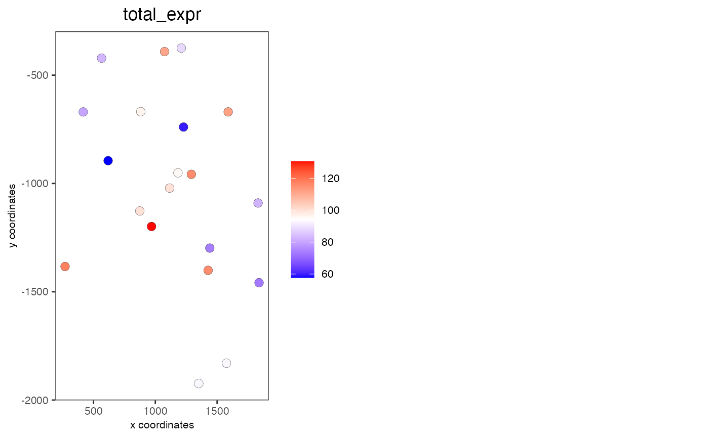
# visualize total expression information
spatCellPlot(mini_giotto_single_cell, cell_annotation_values = 'total_expr')

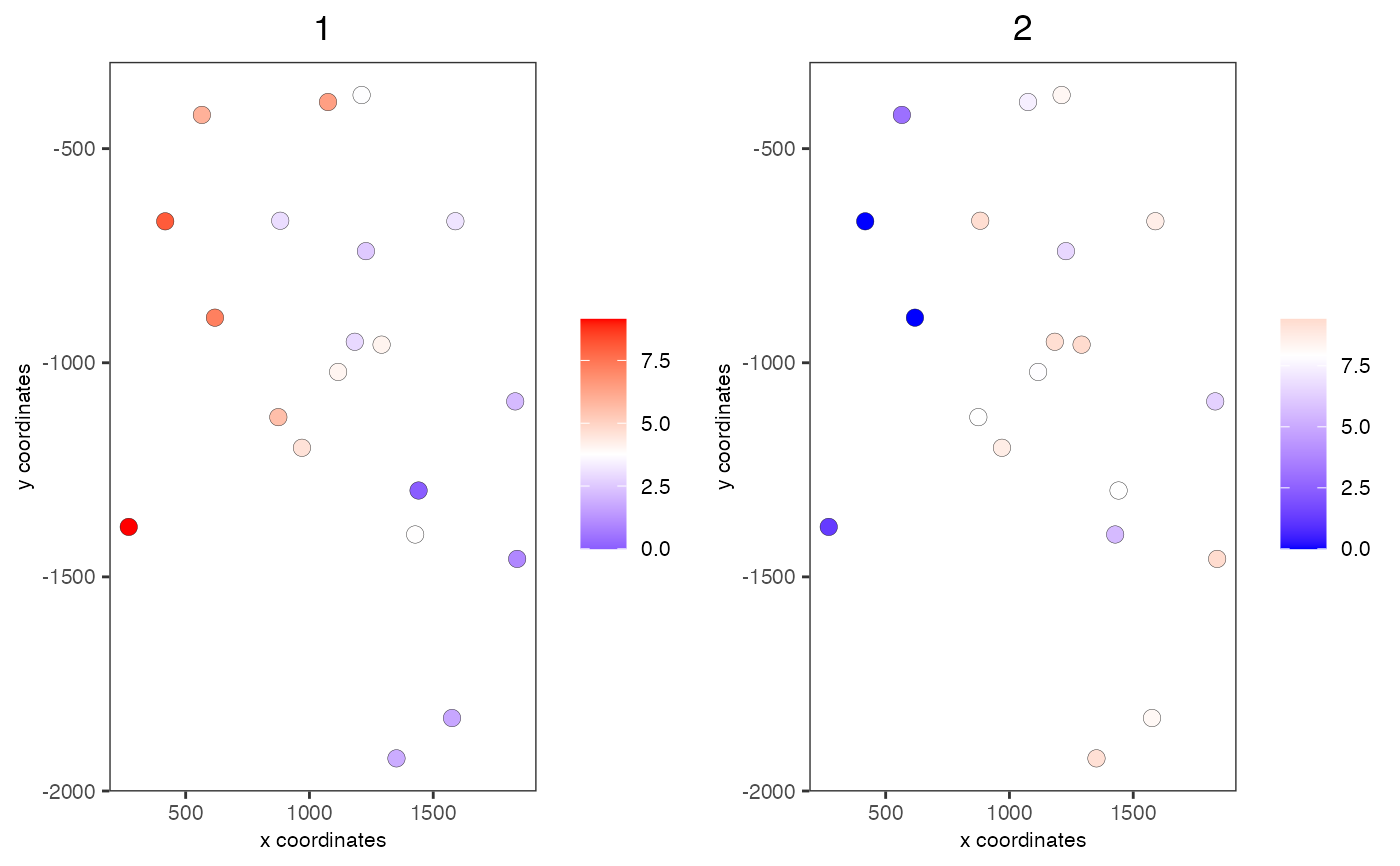
# visualize enrichment results
spatCellPlot(mini_giotto_single_cell,
    spat_enr_names = 'cluster_metagene',
    cell_annotation_values = c('1','2'))